Contents
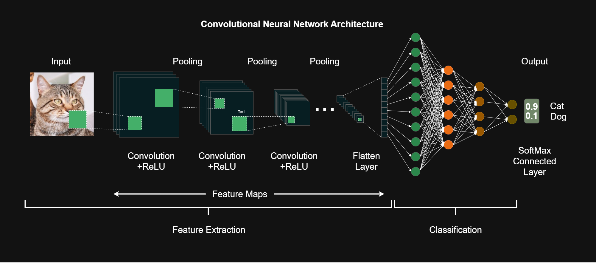
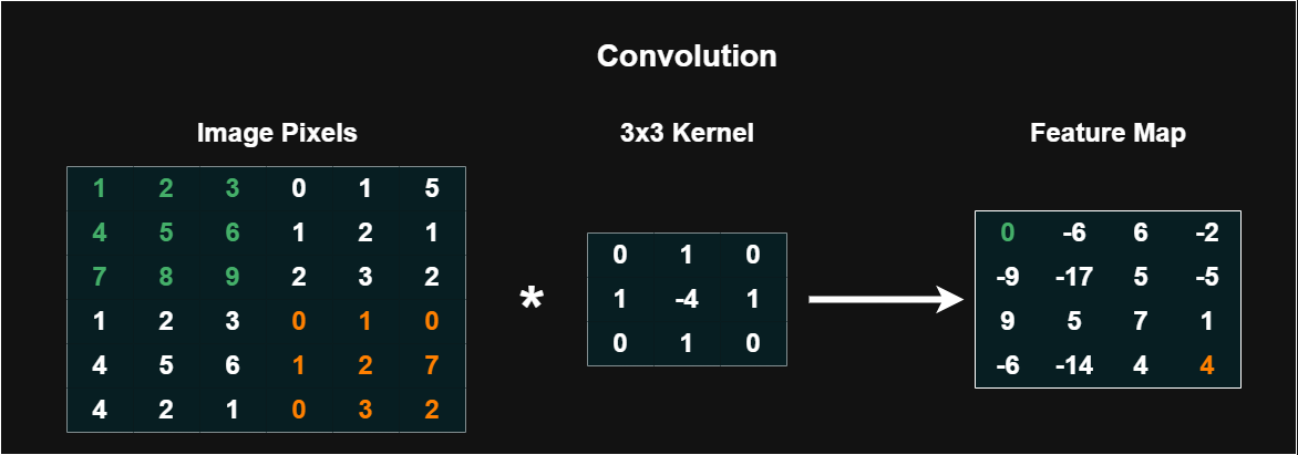
Convolutional layers apply a small matrix, or filter, across an input image to produce a map of responses. Each filter detects a local pattern by computing a weighted sum of the input patch at every position.
In networks that handle color or multi-channel input, the filter extends across all channels, yielding a single feature map per filter. The collection of all feature maps from a layer forms a depth dimension that feeds into the next stage of learning.
The depth of a layer equals the number of filters, a design choice that trades capacity against computation. Commonly, 3x3 filters are used for their balance of expressiveness and efficiency. Padding and stride determine how the spatial dimensions change as the filter slides across the image.
During training, the network learns the filter weights to optimize task performance, shaping the representations that follow layers use. The result is a structured, progressively abstract set of maps that reflect patterns in the data and guide subsequent processing.
This mechanism underpins how a model transforms raw pixels into meaningful features in a practical machine learning workflow.
For a more detailed walk-through on how this works in practice with an example, see Feature Extraction and Convolutional Neural Networks.
Filters in early layers tend to respond to simple patterns such as edges and textures. As the data flows through successive layers, combinations of these patterns form more complex representations, like shapes and object parts. This hierarchical construction enables a model to recognize high-level concepts without explicit programming.
Pooling and stride choices further shape the representation by reducing spatial detail and increasing invariance to small changes in position or illumination. Visualizing feature maps—not as a literal image but as patterns that activate under certain content—offers insight into what the network attends to at different depths.
In practical projects, this hierarchy supports generalization across diverse scenes. When a backbone is pre-trained on large image collections, the early filters often capture universal textures, while later filters adapt to the target task through fine-tuning. The result is a robust, scalable representation that serves as a foundation for many computer vision applications within the machine learning toolkit.
Kernel size: small kernels such as 3x3 are the default due to efficiency and the ability to stack many layers for a larger receptive field. Larger kernels (for example 5x5) cover more area per operation but increase parameters and computation. Stacking small kernels can approximate larger receptive fields with fewer parameters.
Number of filters: more filters per layer increase capacity and the number of distinct patterns captured, but demand more data and compute. In practice, practitioners start with a modest depth and scale up as data and compute allow.
Stride and padding: stride of 1 preserves spatial resolution, while higher strides reduce resolution and perform implicit downsampling. Padding, commonly set to preserve dimensions, prevents loss of border information and keeps feature maps aligned with the input.
Dilation and grouped convolutions: dilation expands the receptive field without increasing parameter count, while grouped convolutions can reduce compute and enable specialized architectures. These are advanced options used in specific design contexts.
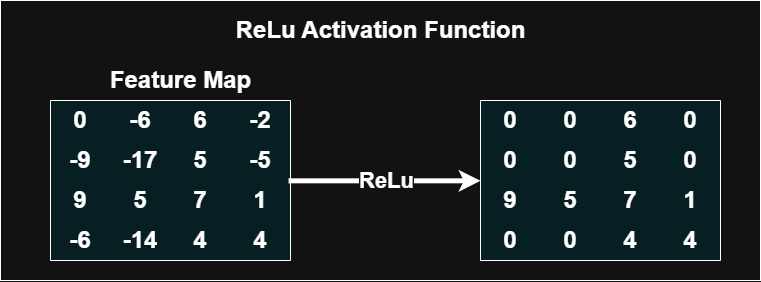
Activation and normalization: nonlinear activations (such as ReLU) enable learning complex patterns, and normalization techniques help stabilize training across a range of batch sizes and data. These choices affect convergence and final accuracy in practical deployments.
Effective practice hinges on data availability and appropriate training strategies. Data augmentation—random flips, rotations, color variations, and crops—helps models generalize when data is limited. Transfer learning, using pre-trained backbones, accelerates development and improves performance on tasks with modest datasets.
In Python programming ecosystems, frameworks such as PyTorch and TensorFlow provide modular implementations for building, training, and evaluating convolutional networks. For deployment, consider inference speed and memory footprint: model quantization, pruning, and optimized runtimes can substantially reduce latency on edge devices without sacrificing accuracy.
These techniques align with digital productivity goals by enabling reliable performance across diverse hardware and use cases.
When selecting a model for a given task, balance architecture depth with available data and compute. A smaller backbone trained with solid augmentation can outperform a larger model trained on a limited dataset. Establish clear benchmarks and monitor both accuracy and inference efficiency during development.
Common challenges include overfitting on small datasets and underfitting when the model capacity is insufficient. Monitoring training and validation curves helps identify these issues early. Regularization strategies, appropriate learning rate schedules, and sufficient augmentation are practical remedies.
Interpreting what the filters and feature maps capture—through visualization of activations or localization methods—provides tangible feedback for model tuning. Techniques such as feature map inspection and localization maps can reveal biases or failure modes, guiding targeted data collection and architectural adjustments.
Interpretability remains a practical concern in production systems. Emphasizing robustness, establishing clear evaluation criteria, and validating performance across representative scenarios support reliable deployment in real-world settings. This approach aligns with disciplined, technology-forward workflows common in modern machine learning practice.
Begin with a well-scoped image classification or detection task and assemble a labeled dataset. Start with a lightweight backbone and a small number of filters to establish a robust baseline. Apply common data augmentations and train on a capable GPU, then evaluate using clear metrics such as accuracy or mean average precision for detection tasks.
Iterate by adjusting kernel sizes, depth, and learning rate schedules, and consider transfer learning if data is modest. Validate on a held-out set and profile inference time for deployment considerations. A disciplined, step-by-step workflow supports steady progress in Python programming environments and translates into reliable, production-ready visual models.
Throughout the process, document decisions, monitor resource usage, and compare alternatives with consistent benchmarks. This structured approach reduces trial-and-error and emphasizes repeatable, actionable results in real-world projects.