TSLA Stock Price Forecasting using LSTM

Stock market forecasting has always been a fascinating challenge for investors, analysts, and researchers.

As stock prices move in complex patterns influenced by numerous factors, predicting future price movements has remained elusive for many years.

However, with advancements in machine learning, particularly the use of Long Short-Term Memory (LSTM) models, predicting stock market trends has become more accessible.

LSTM is a type of Recurrent Neural Network (RNN) that excels at learning from sequential data.

Since the stock market is inherently sequential, with prices depending on past behavior, LSTM models have proven to be highly effective in predicting future trends based on historical data.

What Makes LSTM Ideal for Stock Forecasting?

LSTM networks are designed to process sequences of data.

Unlike traditional machine learning models, LSTMs have the ability to remember information for long periods, making them well-suited for time series forecasting.

In the context of stock market data, an LSTM can look back at past stock prices (often over days, months, or years) and recognize patterns that can provide valuable insights into future price movements.

The key advantage of LSTM models is their capacity to retain important information over time.

Stock prices don’t change in isolation; they are influenced by a variety of factors such as market sentiment, global events, and economic data.

LSTM models can capture these complex relationships in a way that traditional models cannot, enabling them to make more accurate predictions.

Key Considerations in Using LSTM for Stock Forecasting

While LSTM offers a promising approach to forecasting stock prices, several considerations should be taken into account before diving in.

1. Data Quality: The first step in any machine learning project is gathering the right data. For stock forecasting, this typically means historical price data, such as the open, close, high, and low prices, along with trading volume. But data alone isn’t enough; the quality and granularity of the data matter. Data must be cleaned and properly preprocessed to ensure accurate predictions.

2. Time Window: LSTM models perform better when given a window of past data to learn from. In the case of stock prices, this might mean using the last 30 days of price movements to predict the next day’s price. However, the ideal time window (often referred to as time_step) depends on the nature of the stock being analyzed and the frequency of trading data (daily, hourly, etc.).

3. Overfitting: Like any machine learning model, LSTM can suffer from overfitting, especially when the model learns too much from historical data and becomes overly tailored to it. This can make the model ineffective on new, unseen data. Techniques like regularization, dropout layers, and careful tuning of model parameters can help mitigate this risk.

4. Feature Selection: It’s tempting to use a lot of different features, like technical indicators (moving averages, RSI, etc.), sentiment analysis data, or even news articles. While more data can be useful, it’s important to focus on features that genuinely affect stock prices. Too many irrelevant features can overwhelm the model and reduce its performance.

5. Model Evaluation: It’s important to evaluate the performance of the LSTM model not just on training data, but on a separate test set. You can look at metrics like Mean Squared Error (MSE) or Mean Absolute Error (MAE) to assess how well the model is predicting stock prices. Visualizing predictions alongside actual stock prices is also a helpful way to gauge the model’s effectiveness.

The Usefulness of LSTM in Stock Market Forecasting

LSTM-based forecasting models offer several compelling advantages for stock market analysis:

1. Predicting Trends, Not Just Prices: LSTM models are not only good for predicting stock prices for the next day or week but can also help investors identify long-term trends. By capturing patterns in historical data, LSTMs can provide insights into potential upward or downward movements over longer periods, helping investors make strategic decisions.

2. Handling Complex Relationships: The stock market is influenced by a myriad of factors, many of which are non-linear and interdependent. LSTM models can capture these complexities far better than traditional statistical models, which often assume linear relationships between variables.

3. Real-Time Predictions: LSTMs can be updated in real-time with new data, allowing for continuous forecasting. As new stock price data comes in, the model can adjust its predictions to reflect the most current information, making it a valuable tool for day trading and real-time market analysis.

4. Risk Management: Traders and institutions can use LSTM models to better manage risk by forecasting potential price fluctuations and predicting market crashes or bullish trends. By incorporating LSTM models into their decision-making process, traders can gain a more accurate understanding of market behavior.

Limitations and Challenges of LSTM for Stock Forecasting

While LSTM models offer great promise, they are not a magic bullet for predicting stock prices. The following are some limitations and challenges you should be aware of:

• Data Dependency: The performance of an LSTM model heavily depends on the quality and quantity of data. If the historical data is noisy or incomplete, the model’s predictions will likely be unreliable.

• Unpredictable Events: LSTMs are trained on historical data, meaning they are often not equipped to predict unpredictable events like sudden market crashes, geopolitical events, or natural disasters. While LSTMs can forecast trends, they can’t predict black swan events that defy historical patterns.

• Market Efficiency: The Efficient Market Hypothesis (EMH) suggests that stock prices already reflect all available information, meaning forecasting stock prices might be inherently impossible. While LSTM models can often find patterns that humans cannot, it’s worth considering that some degree of unpredictability is built into the market.

Stock Forecasting with Python

You can find all the code on GitHub.

Set Up the Environment

To forecast stock prices with LSTM, you’ll need Python along with a few essential libraries. In your python environment, install the following libraries:

pip install numpy pandas matplotlib scikit-learn tensorflow yfinance

Once the libraries have been installed, add the following import to your .ipynb jupyter notebook.

# Import necessary libraries
import pandas as pd
import matplotlib.pyplot as plt
from sklearn.preprocessing import MinMaxScaler
from tensorflow.keras.models import Sequential
from tensorflow.keras.layers import LSTM, Dense
from datetime import datetime
import yfinance as yf
from sklearn.preprocessing import MinMaxScaler
import numpy as np

Prepare Data

We’ll use historical data from Yahoo Finance to apply our strategy. For this example, let’s use Tesla’s stock (TSLA).

# Define the stock symbol and the date range for our data
stock_symbol = 'TSLA'
start_date = '2016-01-01'
end_date = datetime.today().strftime('%Y-%m-%d')  # Sets end date to today's date
print(f"Ticker: {stock_symbol}\nStart Date: {start_date}\nEnd Date: {end_date}")

After downloading the data, we can now preprocess it for easy forecasting:

df = yf.download(stock_symbol, start=start_date, end=end_date)

# Select the desired columns (first level of MultiIndex)
df.columns = df.columns.get_level_values(0)
# Keep only the columns you are interested in
df = df[['Open', 'Close', 'Volume', 'Low', 'High']]
# If the index already contains the dates, rename the index
df.index.name = 'Date'  # Ensure the index is named "Date"
    
# Resetting the index if necessary
df.reset_index(inplace=True)
# Ensure that the index is of type datetime
df['Date'] = pd.to_datetime(df['Date'])
# Set the 'Date' column as the index again (in case it's reset)
df.set_index('Date', inplace=True)
df.head()

Visualize the Chart

# Plot the closing price over time
plt.figure(figsize=(14, 7))
plt.plot(df['Close'], label='Closing Price')
plt.title('Tesla Stock Closing Price Over Time')
plt.xlabel('Date')
plt.ylabel('Price')
plt.legend()
plt.grid(True)
plt.show()

TSLA Closing Price Visualization

Scale the Data

In this step, we extract the Close prices for forecasting and reshape the data to a 2D array. The MinMaxScaler is then used to normalize the data, scaling it to a range between 0 and 1 to prepare it for training the model.

# Use the 'Close' prices for forecasting
data = df['Close'].values

# Reshape the data to 2D array (required for MinMaxScaler)
data = data.reshape(-1, 1)

# Normalize the data using MinMaxScaler
scaler = MinMaxScaler(feature_range=(0, 1))
scaled_data = scaler.fit_transform(data)

Data Split

The dataset is split into training (80%) and testing (20%) sets. A function is defined to prepare the data for the LSTM model by creating sequences of 30 previous days’ prices to predict the next day’s price. The data is then reshaped into 3D arrays to match the LSTM input format.

# Split the data into training and test sets (80% training, 20% testing)
train_size = int(len(scaled_data) * 0.8)
train_data, test_data = scaled_data[:train_size], scaled_data[train_size:]

# Create a function to prepare the data for LSTM
def create_dataset(data, time_step):
    X, y = [], []
    for i in range(len(data) - time_step - 1):
        X.append(data[i:(i + time_step), 0])
        y.append(data[i + time_step, 0])
    return np.array(X), np.array(y)

# Prepare training and testing data
time_step = 30  # Using 30 previous days to predict the next one
X_train, y_train = create_dataset(train_data, time_step)
X_test, y_test = create_dataset(test_data, time_step)

# Reshape the data into 3D array for LSTM input (samples, time steps, features)
X_train = X_train.reshape(X_train.shape[0], X_train.shape[1], 1)
X_test = X_test.reshape(X_test.shape[0], X_test.shape[1], 1)

X_train.shape, X_test.shape

Build the LSTM Model

An LSTM model is built with two LSTM layers, each having 50 units. The first layer returns sequences to feed into the second layer, while the output layer uses the ReLU activation function to ensure non-negative predictions. The model is compiled using the Adam optimizer and mean squared error loss. The model summary is displayed to show the architecture.

# Build the LSTM model
model = Sequential()

# First LSTM layer
model.add(LSTM(units=50, return_sequences=True, input_shape=(X_train.shape[1], 1)))

# Second LSTM layer
model.add(LSTM(units=50, return_sequences=False))

# Output layer with ReLU activation to ensure non-negative predictions
model.add(Dense(units=1, activation='relu'))  # ReLU prevents negative predictions

# Compile the model
model.compile(optimizer='adam', loss='mean_squared_error')

# Summarize the model
model.summary()

Begin Training

The model is trained using the training data for 50 epochs with a batch size of 32. Validation data (test set) is provided to monitor performance during training and prevent overfitting.

# Train the LSTM model
history = model.fit(X_train, y_train, epochs=50, batch_size=32, validation_data=(X_test, y_test))

# Save the trained model to a file
model.save(f'{stock_symbol}_lstm_stock_model.h5')

print("Model saved successfully!")

Visualize Training Results

# Plot training and validation loss
plt.figure(figsize=(10, 6))
plt.plot(history.history['loss'], label='Training Loss', color='blue')
plt.plot(history.history['val_loss'], label='Validation Loss', color='orange')

# Customize the plot
plt.title('Training and Validation Loss Over Epochs')
plt.xlabel('Epochs')
plt.ylabel('Loss')
plt.legend()
plt.grid(True)

# Show the plot
plt.show()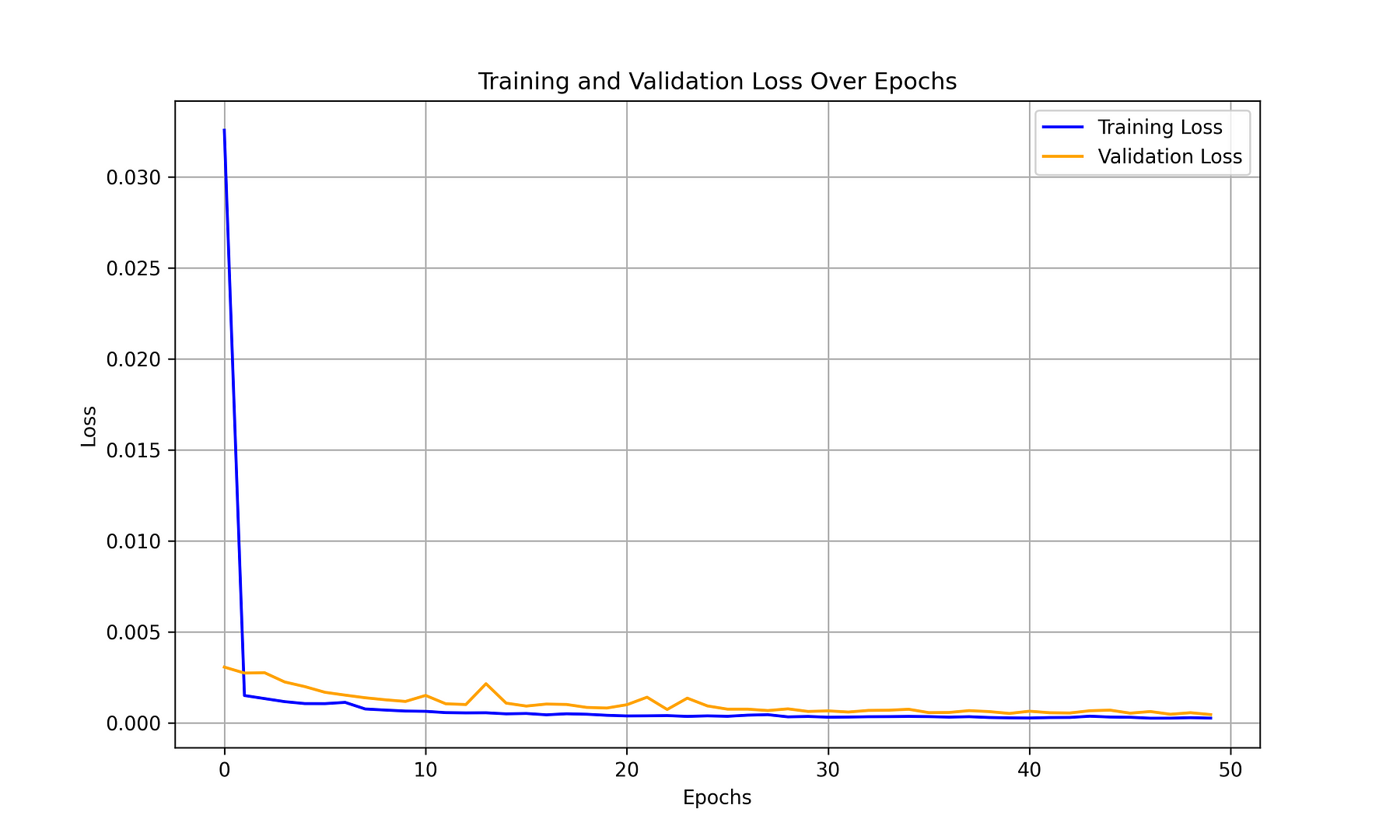

Training Results Plot

Predict Future Data

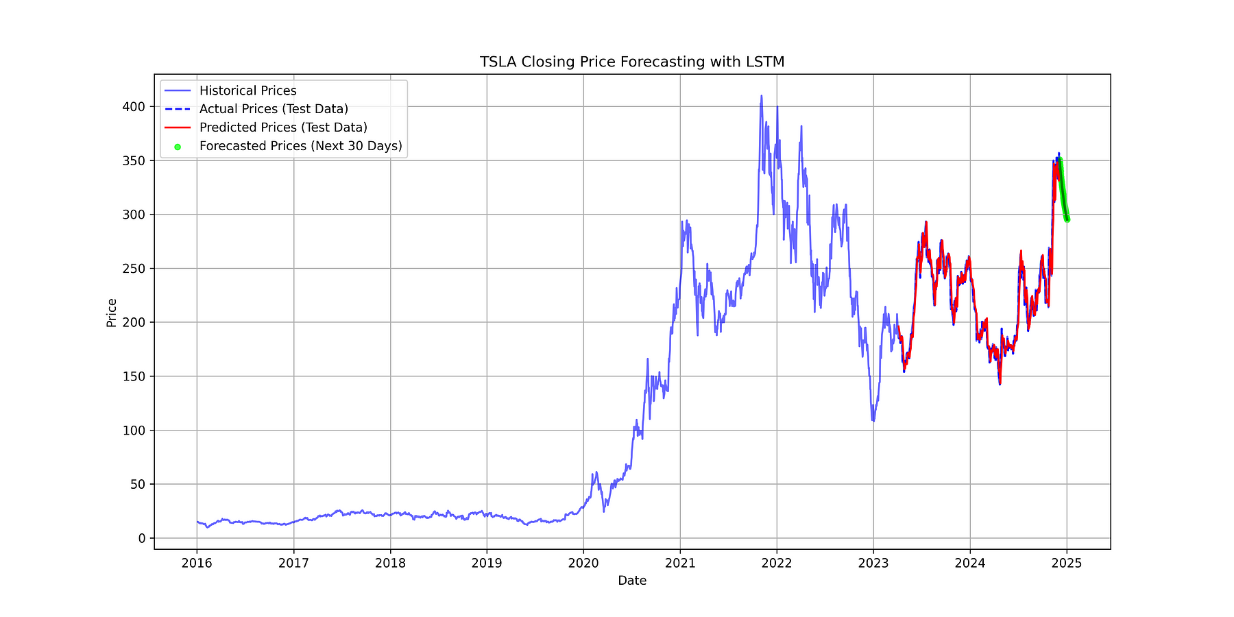
The model predicts stock prices on the test data, and both predicted and actual values are inverse-transformed to their original scale. Additionally, the model forecasts the next 30 days of stock prices using the most recent data, with each prediction used to update the input for subsequent forecasts.

# Predict on the test data
predicted_prices = model.predict(X_test)

# Inverse transform the predictions and actual values to get the original scale
predicted_prices = scaler.inverse_transform(predicted_prices)
y_test_actual = scaler.inverse_transform(y_test.reshape(-1, 1))

# Forecast
last_n_days = scaled_data[-time_step:].reshape(1, -1)
last_n_days = last_n_days.reshape((last_n_days.shape[0], last_n_days.shape[1], 1))

next_n = 30

predicted_next_n = []
for _ in range(next_n):
    next_day = model.predict(last_n_days)
    predicted_next_n.append(next_day[0, 0])
    last_n_days = np.append(last_n_days[:, 1:, :], next_day.reshape(1, 1, 1), axis=1)

predicted_next_n = scaler.inverse_transform(np.array(predicted_next_n).reshape(-1, 1))

Plot the Prediction Results

# Plot the historical data and forecasted target data
plt.figure(figsize=(14, 7))

# Plot the full historical closing prices
plt.plot(df.index, data, label='Historical Prices', color='blue', alpha=0.6)

# Plot the actual closing prices from test data (this part will be part of the full data)
plt.plot(df.index[-len(y_test_actual):], y_test_actual, label='Actual Prices (Test Data)', color='blue', linestyle='--')

# Plot the predicted prices from the model (for test data)
plt.plot(df.index[-len(predicted_prices):], predicted_prices, label='Predicted Prices (Test Data)', color='red')

# Post-process the forecasted values to make sure they are non-negative
predicted_next_n[predicted_next_n < 0] = 0  # Prevent negative forecasted prices

# Plot the forecasted prices
forecast_dates = pd.date_range(df.index[-1], periods=next_n+1, freq='D')[1:]  # Generate dates for the forecast
plt.scatter(forecast_dates, predicted_next_n, label=f'Forecasted Prices (Next {next_n} Days)', color='lime', s=20, alpha=0.7)
plt.plot(forecast_dates, predicted_next_n, color='green', linestyle='-', linewidth=2)

# Customize the plot
plt.title(F'{stock_symbol} Closing Price Forecasting with LSTM')
plt.xlabel('Date')
plt.ylabel('Price')
plt.legend()
plt.grid(True)

# Save plot in 300 dpi
plt.savefig(f'{stock_symbol}_forecast.png', dpi=300)

# Show the plot
plt.show()

TSLA Stock Price with Forecast on Test Data and a Future Period

Conclusion

Stock market forecasting with LSTM is a powerful approach that leverages deep learning to uncover hidden patterns in time series data.

By understanding the nuances of LSTM and considering key factors like data quality, model evaluation, and overfitting, investors can harness the power of this technology to gain an edge in the market.

However, like any tool, LSTM should be used cautiously and responsibly, keeping in mind the limitations and uncertainties inherent in financial markets.