Sample Training Images

What is YOLO?

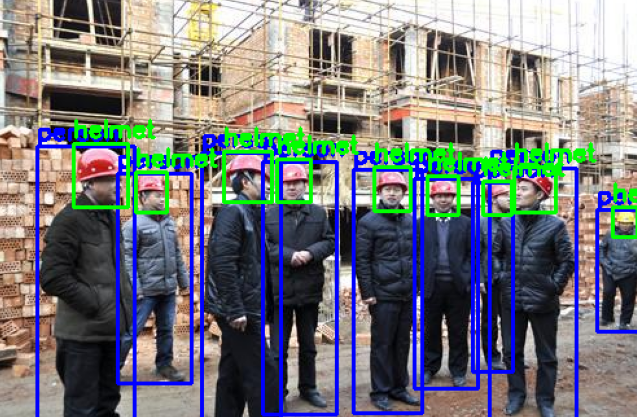
YOLO (You Only Look Once) is a deep learning-based object detection algorithm known for its speed and accuracy. Unlike traditional models that process images in multiple steps, YOLO detects objects in a single pass, making it one of the most efficient detection models for real-time applications. It is widely used in autonomous driving, surveillance, and medical imaging, where fast and accurate detection is essential.

You can explore the foundational paper by Joseph Redmon and colleagues, titled You Only Look Once: Unified, Real-Time Object Detection.

In this article, we will fine-tune YOLO11 on a Kidney Stones dataset formatted in the YOLO annotation format. The goal is to adapt an existing YOLO model to accurately detect kidney stones in medical images. Instead of training a model from scratch, we will leverage transfer learning to make the most of pre-trained knowledge while adapting the model to this specific medical task.

1. Why Not Train a Model from Scratch?

Object detection models are typically built using Convolutional Neural Networks (CNNs). While training a CNN from scratch is possible, it comes with several challenges:

• Requires Large Datasets – Training a deep CNN requires millions of labeled images, which is often unrealistic for specialized fields like medical imaging.

• Computationally Expensive – Training from scratch can take weeks or even months on high-end GPUs.

• Complex Hyperparameter Tuning – Choosing the right learning rate, batch size, and weight initialization requires extensive experimentation.

• Risk of Overfitting – With limited data, a model trained from scratch may memorize the training images instead of learning meaningful patterns.

For most real-world applications, fine-tuning a pre-trained model is a more practical approach.

2. Why Fine-Tune YOLO Instead?

Fine-tuning is a technique in transfer learning, where a model that has already learned general object detection features is adapted to a new dataset. Instead of learning from scratch, the model retains its previously learned low-level features (edges, textures) and high-level structures (shapes, objects) while adjusting to the new task.

Fine-tuning YOLO offers several advantages:

• Faster Training – Since the model already understands general image features, fewer training epochs are required.

• Works Well with Limited Data – Fine-tuning can produce high-quality models even with relatively small datasets.

• Improved Accuracy – The model retains useful prior knowledge while adapting to new objects.

• Lower Computational Cost – Only specific layers are updated, reducing hardware requirements.

Training from scratch is only necessary when working with a completely new domain, requiring a custom architecture or an extremely large dataset. In most cases, fine-tuning a pre-trained YOLO model is the best approach.

3. How YOLO Works

YOLO is a single-stage object detection algorithm that performs object localization and classification in a single forward pass through the network. This design makes YOLO extremely fast compared to traditional two-stage detectors like Faster R-CNN.

YOLO Architecture, Diagram Adapted from the Original Paper

Here's a breakdown of how YOLO works:

1. Input Image Processing

   The input image is first resized to a fixed dimension (448x448) and then normalized. This allows the model to process images of varying sizes while maintaining consistent output dimensions.

2. Grid-Based Detection

   YOLO divides the input image into an S × S grid (e.g., 13×13 or 16×16). Each grid cell is responsible for detecting objects whose centers fall inside that cell.

3. Bounding Box and Class Predictions

   Each grid cell predicts:

   • B bounding boxes, each defined by 4 coordinates: center x, center y, width, and height — all relative to the grid cell and normalized to the image dimensions.

   • A confidence score for each bounding box, representing the likelihood that a box contains an object and how accurate the bounding box is (based on IoU with the ground truth).

   • Class probabilities for each of the C classes (e.g., person, car, dog), typically using a softmax or sigmoid activation.

   So, for every grid cell, the model outputs:

   Plaintext

   B × (5 + C) values 

   Where:

   • 5 = (x, y, w, h, object confidence)

   • C = number of classes

4. Decoding Predictions

   The model's raw output is decoded into bounding boxes and class scores. At this stage, many boxes may overlap or refer to the same object.

5. Non-Maximum Suppression (NMS)

   YOLO uses Non-Maximum Suppression (NMS) to remove duplicate boxes and retain only the most confident predictions. NMS works by:

   • Keeping the box with the highest confidence score for a class.

   • Removing any boxes that have high IoU overlap (e.g., > 0.5) with the selected box.

6. Final Output

   After NMS, YOLO returns the final set of bounding boxes with associated class labels and confidence scores, making it suitable for real-time detection tasks.

4. Fine-Tuning YOLO for Kidney Stone Detection

Detecting kidney stones in medical images is a challenging task. Unlike objects in common datasets like COCO, kidney stones are often small, blend into the background, and require expert annotation. Fine-tuning a YOLO model allows us to adapt it to this specialized task.

Challenges in kidney stone detection include:

• Small Object Size – Kidney stones are tiny, making them harder to detect.

• Similar Background Features – Medical images often contain noise and artifacts that make detection difficult.

• Limited Annotated Data – Medical datasets are smaller than general-purpose datasets due to the complexity of annotation.

Pre-trained YOLO models are optimized for detecting objects like cars, people, and animals but not kidney stones. Fine-tuning helps us transfer learned object detection knowledge to this domain, improving accuracy while avoiding the need for extensive data and computing resources.

Setting Up the Environment

Before training our YOLO11 model to detect kidney stones, we need to set up the right Python environment. In this section, we will use Google Colab, a free, browser-based tool that lets you write and run Python code in the cloud.

All the code used in this guide can be found on the Colab Notebook and also on this GitHub Repository. Feel free to improve and adapt the code for your own use case.

1. What is Google Colab?

Google Colab (short for "Colaboratory") is a cloud-based notebook platform provided by Google. It is similar to Jupyter Notebooks but runs entirely in your web browser. With Colab, you can:

• Write and execute Python code

• Use free GPU and TPU hardware for faster computations

• Upload and manage files directly in the interface

• Save notebooks to Google Drive or GitHub

This makes it a great choice for training deep learning models like YOLO, especially for beginners or those without access to a local GPU.

2. Creating a New Notebook

To get started, go to https://colab.research.google.com and sign in with your Google account.

Google Colab Signin Page

Once you're in, click on New Notebook in the bottom-right corner. This will create a blank notebook where you can begin writing Python code.

You can rename your notebook by clicking on the default title at the top (for example, rename it to kidney_stones_yolo.ipynb).

Rename Notebook

3. Enabling GPU Support

Training object detection models is computationally intensive, so we’ll enable GPU acceleration to speed up the process. Here’s how:

In the notebook menu bar, click on Runtime, then select Change runtime type. In the window that appears, set the Hardware accelerator to GPU, then click Save.

This gives your notebook access to a virtual GPU hosted by Google — no extra setup required.

Select GPU Runtime

4. Installing the Ultralytics Library

Next, we’ll install the ultralytics package, which includes YOLO11 and provides a simple interface for training and evaluating YOLO models. This library makes it easy to fine-tune a model with just a few lines of code.

In your first code cell, type and run the following command:

%pip install ultralytics 

This command installs everything needed to train and test YOLO models, including utility functions and pre-trained weights.

5. Importing Required Libraries

Now that the main library is installed, we’ll import several Python packages that will help us load images, process data, and display results. These libraries will be used throughout the training and evaluation process.

In a new code cell, add the following imports:

import kagglehub
import os
import random
import cv2
import glob
import matplotlib.pyplot as plt
import matplotlib.image as mpimg

Here’s a brief explanation of what each library does:

• kagglehub: Allows us to download datasets and models directly from Kaggle into our notebook environment.

• os: Provides tools for working with the file system—used to build file paths, navigate directories, and check for file existence.

• random: Helps us randomly select images or data samples, useful for visualization or splitting data.

• cv2 (OpenCV): A powerful library for image processing. In this project, it's used to read, convert, and annotate images.

• glob: Makes it easy to find files matching a specific pattern (e.g., all .jpg files in a folder), which is helpful when loading datasets or predictions.

• matplotlib.pyplot and matplotlib.image: Used together to display images, plot training results, and visualize prediction outputs directly within the notebook.

You don’t need to memorize these libraries right now. We’ll explain each one in context as we move forward.

Dataset Overview

1. Dataset Description

In this project, we will be using a specialized dataset focused on kidney stones detection. The Kidney Stone Images with Bounding Box Annotations dataset provides a valuable resource for improving detection algorithms in medical imaging. The images are derived from CT scans and cover different aspects of kidney stones, such as their location, size, and shape. The accompanying bounding box annotations are critical for teaching AI models to recognize kidney stones accurately.

Researchers and healthcare professionals can leverage this dataset to create AI models that can aid in diagnosing kidney stones faster and more accurately, contributing to the development of telemedicine solutions and more efficient healthcare tools.

This dataset can be found on Kaggle, where it is made available for free for research and educational purposes. You can access the dataset by visiting Kaggle's Kidney Stone Dataset. It provides a valuable resource for training AI models to detect kidney stones in medical imaging, with proper annotations.

2. Downloading the Dataset

To begin working with this dataset, we can use Kaggle Hub to download the dataset. Kaggle Hub allows you to easily access datasets directly into your environment.

The code snippet below downloads the latest version of the dataset:

# Download latest version
path = kagglehub.dataset_download("safurahajiheidari/kidney-stone-images")

print("Path to dataset files:", path)

This code downloads the dataset to your environment, and the path variable will store the directory where the files are located.

Once downloaded, you can list the files in the dataset folder to explore its structure. Use the following command to view the contents:

os.listdir(path) 

The output should look like this:

['README.dataset.txt', 'README.roboflow.txt', 'data.yaml', 'valid', 'test', 'train'] 

Here’s what each folder and file represents:

• README.dataset.txt and README.roboflow.txt: These are documentation files containing details about the dataset.

• data.yaml: This file contains metadata, including the class names and paths to training, validation, and test images.

• train: Contains the training images and their corresponding annotations.

• valid: Contains validation images used to evaluate the model during training.

• test: Contains test images used to assess the model's final performance.

3. Dataset Statistics

The dataset, contains a total of 1,300 images that are specifically tailored for kidney stone detection in medical imaging. Each image is annotated in YOLOv8 format, which is widely used in the computer vision community for object detection tasks. These annotations help indicate the exact location of kidney stones in the images by using bounding boxes.

In terms of dataset preprocessing, a few augmentations were applied to increase the robustness of the dataset for model training:

• 50% Probability of Horizontal Flip: This means each image has a 50% chance of being flipped horizontally, creating a mirrored version of the original image.

• Random Rotation Between -10 and +10 Degrees: The images are randomly rotated by an angle between -10 and +10 degrees. This introduces slight variations to the images to help the model generalize better.

The dataset is well-structured with folders dedicated to different stages of the model training process. After downloading the dataset, you will find the following key components:

• Images: The images themselves, stored in the train, valid, and test folders. Each folder contains the respective images used for training, validation, and testing the model.

• Annotations: Each image has a corresponding annotation file (in YOLO format) that provides information about the location of kidney stones in the image.

This dataset, along with its annotations and augmentations, provides a solid foundation for fine-tuning object detection models like YOLO, especially for medical applications where accurate detection is crucial. By utilizing this dataset, you can significantly enhance your model's performance in detecting kidney stones across various medical images.

4. Visualizing Random Images from the Training Set

Now that we have the dataset, let’s take a quick look at some sample images and their annotations. This will help us understand the format and ensure everything is set up correctly.

The following code snippet selects six random images from the train folder, displays them in a 2x3 grid, and overlays the corresponding bounding boxes on each image.

split = "train"

# Construct image and label paths
image_folder = os.path.join(path, split, "images")
label_folder = os.path.join(path, split, "labels")

# Get a list of image files
image_files = [f for f in os.listdir(image_folder)]

# Select 6 random images
random_images = random.sample(image_files, 6)

# Create a 2x3 grid for visualization
fig, axes = plt.subplots(2, 3, figsize=(15, 10))

for i, ax in enumerate(axes.flat):
    image_path = os.path.join(image_folder, random_images[i])

    # Read the image
    image = cv2.imread(image_path)
    image = cv2.cvtColor(image, cv2.COLOR_BGR2RGB)  # Convert to RGB

    # Read the corresponding YOLO annotation file
    label_file = os.path.join(label_folder, random_images[i].replace(".jpg", ".txt"))

    # Get image dimensions
    height, width, _ = image.shape

    # Read bounding box annotations
    if os.path.exists(label_file):
        with open(label_file, "r") as f:
            for line in f:
                values = line.strip().split()
                class_id = int(values[0])  # First value is class ID
                x_center, y_center, bbox_width, bbox_height = map(float, values[1:])

                # Convert YOLO format to bounding box coordinates
                x_min = int((x_center - bbox_width / 2) * width)
                y_min = int((y_center - bbox_height / 2) * height)
                x_max = int((x_center + bbox_width / 2) * width)
                y_max = int((y_center + bbox_height / 2) * height)

                # Draw bounding box
                rect = plt.Rectangle((x_min, y_min), x_max - x_min, y_max - y_min, fill=False, edgecolor=(0, 1, 0), linewidth=2)
                ax.add_patch(rect)

    ax.imshow(image)
    ax.axis("off")

plt.tight_layout()
plt.show()

This code will display six random training images along with their bounding boxes, allowing you to visually inspect the data and make sure everything is labeled correctly.

Sample Training Images

With this, you’ve explored the dataset and confirmed that it’s ready for training. In the next section, we’ll dive into fine-tuning the YOLO model for kidney stone detection.

Fine-tune the YOLO Model

Now that we have set up our environment and reviewed the dataset, we are ready to fine-tune the YOLO11 model on the kidney stone detection task. This section will guide you through training the model using the data we've prepared.

1. Training the Model

Fine-tuning a pre-trained YOLO model is straightforward with the ultralytics library. We will use the YOLO11n model, the smallest version of the YOLO11 series that is optimized for smaller datasets and faster computations.

Other versions include:

The training command is as follows:

!yolo task=detect mode=train model=yolo11n.pt data={path}/data.yaml epochs=50 imgsz=416 plots=True

• task=detect: This indicates that we are performing an object detection task.

• mode=train: Specifies that we want to train the model.

• model=yolo11n.pt: This is the pre-trained YOLO11 model that we will fine-tune.

• data={path}/data.yaml: The path to the data configuration file that points to the training, validation, and test datasets.

• epochs=50: The number of training epochs (iterations over the entire dataset).

• imgsz=416: Specifies the image size to resize the input images to during training.

• plots=True: Enables the plotting of performance metrics like training loss and accuracy.

2. Training Output

Once you execute this command, the model will begin training. The training process will output various logs and metrics that we can use to monitor its progress. These logs typically include:

• Training Loss: The loss at each epoch, which measures how well the model is fitting the data.

• Metrics: Such as precision, recall, and mean average precision (mAP), which give us an idea of how well the model is performing in detecting kidney stones.

Here’s an example of the output from the training process:

Example Training Output for the First 5 Epochs

As the training progresses, you should see a reduction in the loss values and an improvement in the detection accuracy.

3. Training Results

After training the YOLO model, we can visualize the training metrics—such as classification loss, localization loss, precision, and recall—over time. This helps us evaluate how well the model is learning and whether we need to adjust hyperparameters like the learning rate or number of epochs.

The plot below shows how these metrics evolved during training:

# Path to the results image
image_path = f'/content/runs/detect/train/results.png'

# Read the image using matplotlib
img = mpimg.imread(image_path)

# Display the image using matplotlib
plt.figure(figsize=(10, 8))
plt.imshow(img)
plt.axis('off')  # Hide the axes

# Save the image with tight bounding box to remove padding
plt.savefig("training_results.png", bbox_inches='tight', pad_inches=0)

# Show the image
plt.show()

print(f"Displayed: {image_path}")

YOLO Training Results

Evaluate the Model

After training the YOLO model on our kidney stone detection dataset, the next critical step is to evaluate its performance on unseen data. This involves running the model on test images that were not part of the training or validation process to assess how well it generalizes to new examples. In practical terms, this helps us understand whether the model can reliably detect kidney stones in real-world medical images.

1. Running the Model on the Test Set

Once training is complete, we use the best-performing model weights saved during training to make predictions on the test dataset. The following command is used to run YOLO on the test images:

!yolo task=detect mode=val model=/content/runs/detect/train/weights/best.pt data={path}/data.yaml split=test 

Let’s break down what this command does:

• task=detect: Specifies that we are performing object detection.

• mode=val: Runs the model in evaluation mode, computing metrics like precision, recall, and mean average precision (mAP) on the test split.

• model=...: Points to the best model weights obtained during training.

• data=...: Specifies the path to the dataset configuration file.

• split=test: Instructs the model to evaluate on the test subset of the data.

This command not only runs the predictions but also generates quantitative metrics to summarize the model’s performance.

2. Evaluation Metrics

When the model is evaluated on the test set, the following metrics are printed:

Here’s what each of these means:

• Images: The number of test images evaluated (123 in this case).

• Instances: Total number of annotated objects (224 kidney stones).

• Precision (P = 0.815): Out of all predicted bounding boxes, 81.5% correctly matched a ground truth object. This indicates that the model is good at avoiding false positives.

• Recall (R = 0.687): Out of all actual kidney stones, the model correctly identified 68.7%. While this is solid, it suggests there is still room to reduce false negatives.

• mAP@0.5 (0.705): The mean Average Precision at an IoU threshold of 0.5 is 70.5%, showing that the model is fairly accurate at detecting and localizing objects.

• mAP@0.5:0.95 (0.315): The mean Average Precision averaged over IoU thresholds from 0.5 to 0.95. A value of 31.5% indicates that while the model performs well on easier detection tasks, it struggles with more precise localization.

These results suggest the model performs reasonably well for a single-class medical detection task. It strikes a good balance between precision and recall, which is important in medical imaging where both false positives and false negatives can have consequences.

Make Predictions

Once the YOLO model has been trained and evaluated, the next step is to use it for real-world inference—predicting kidney stones on unseen medical images. This is where the model becomes truly useful, whether in research, clinical applications, or deployment scenarios.

To make predictions, we’ll use the model weights saved during training. The command below runs inference on a set of test images:

!yolo task=detect mode=predict model=/content/runs/detect/train/weights/best.pt conf=0.25 source={path}/test/images save=True

Let’s break this down:

• task=detect: Specifies that we are performing object detection.

• mode=predict: Tells YOLO to generate predictions on new, unseen data.

• model=...: Path to the best model weights saved during training.

• conf=0.25: Sets a confidence threshold. Predictions below this value will be discarded.

• source=...: Directory containing the test images.

• save=True: Ensures that the predicted images (with bounding boxes) are saved to disk for inspection.

After running this command, YOLO will create a new directory (e.g., /runs/detect/predict2) where all the annotated predictions are stored.

💡 Tip: You can reuse this model later for inference on completely new images simply by modifying the source path. This makes it possible to deploy the model in production workflows or embed it in other systems.

Visualizing Predictions

To assess how well the model performs visually, it’s helpful to display a few of the predicted images. Below is a script that loads the latest set of prediction results and displays the first six images in a 2×3 grid:

# Get the latest prediction folder
latest_folder = max(glob.glob(f'/content/runs/detect/predict*/'), key=os.path.getmtime)

# Get the image paths
image_paths = glob.glob(f'{latest_folder}/*.jpg')[:6]  # Fetch 6 images for the grid

# Create a 2x3 grid
fig, axes = plt.subplots(2, 3, figsize=(15, 10))

# Flatten the axes array to make it easier to iterate
axes = axes.flatten()

# Loop over the images and axes
for i, img_path in enumerate(image_paths):
    img = mpimg.imread(img_path)  # Read the image using matplotlib
    
    ax = axes[i]  # Select the corresponding axis
    ax.imshow(img)
    ax.axis('off')  # Hide the axes
    ax.set_title(f"Image {i+1}")  # Optional: Set the title for each image

# Adjust layout to prevent overlap
plt.tight_layout()

plt.savefig("model_inference_images.png")

# Show the grid of images
plt.show()

# Print the paths of the displayed images
for img_path in image_paths:
    print(f"Displayed: {img_path}")

This script automatically finds the most recent prediction folder and displays six of the saved images. Each image will show the detected kidney stones with bounding boxes, allowing you to visually verify the model’s predictions.

Kidney Stone Detection Results (Predicted Images)

Conclusion and Future Work

In this project, we successfully fine-tuned a YOLO11 model for the detection of kidney stones in medical images. By leveraging a pre-trained model and fine-tuning it on a specialized dataset, we were able to significantly reduce the time and computational resources required for training, while also achieving strong detection performance.

As with any machine learning project, there is always room for improvement. Some potential areas for future work include:

• Increasing the dataset size: While our model performed well on the available data, having more labeled images could further improve its accuracy.

• Data Augmentation: Applying additional data augmentation techniques, such as random cropping or color variations, could help the model generalize better to unseen data.

• Model Improvements: Exploring other variants of the YOLO architecture, such as YOLOv4 or YOLOv5, could potentially lead to better performance.

• Using Larger YOLOv11 Variants: In this article, we used yolov11n, the smallest and fastest model optimized for speed and low computational cost. For higher accuracy, especially in complex medical tasks, consider switching to a larger variant like yolov11x. These models offer deeper architectures and more parameters, often leading to improved detection performance—though they require more computational resources.

This work demonstrates the power of transfer learning and the efficiency of the YOLO model for medical imaging tasks like kidney stone detection. By fine-tuning an existing model, we were able to achieve high detection accuracy without the need for massive computational resources or extensive labeled data.

💡Remember, all the code used in this guide can be found on the Colab Notebook and also on this GitHub Repository. Feel free to improve and adapt the code for your own use case.