Before And After Non Maximum Suppression

In object detection tasks, models often return multiple bounding boxes around a single object. These overlapping predictions can lead to ambiguity in the final output.

Non-Maximum Suppression (NMS) is a critical post-processing step used to filter these predictions, ensuring that only the most relevant bounding boxes are retained.

In this comprehensive guide, we will examine the problem NMS is designed to solve, explore the algorithm in detail, and walk through a step-by-step implementation using Python.

By visualizing bounding boxes before and after applying NMS, you will gain a practical understanding of its impact and how it improves the quality of object detection outputs.

Why Do We Need Non-Maximum Suppression?

Object detection models such as YOLO, SSD, and Faster R-CNN work by predicting multiple bounding boxes with associated confidence scores. When a model detects an object, it often produces several overlapping boxes, each with a slightly different position and score.

This redundancy is expected, it provides robustness, but we need a way to eliminate unnecessary predictions.

NMS ensures that only the highest-quality predictions remain, removing overlapping boxes that likely refer to the same object. This is essential for clarity, performance, and downstream applications such as object tracking, classification, or visualization.

The Problem: Multiple Overlapping Predictions

To better understand the issue, consider a detector that identifies a single object but produces multiple bounding boxes for it:

• Each box has a confidence score indicating the model’s certainty.

• The boxes often overlap significantly, especially when the object is well-centered in the image.

• Without post-processing, all of these predictions may be kept, cluttering the result.

This is where Non-Maximum Suppression becomes essential.

What is Non-Maximum Suppression (NMS)?

Non-Maximum Suppression is a filtering algorithm that reduces redundant bounding boxes in object detection. Its purpose is to retain only the most confident detections while suppressing others that have a significant overlap with them.

The NMS Algorithm (Step-by-Step):

1. Sort all predicted bounding boxes by their confidence scores in descending order.

2. Select the bounding box with the highest confidence score.

3. Compute the Intersection over Union (IoU) between this box and all other boxes.

4. Remove boxes that have an IoU greater than a predefined threshold (e.g., 0.5).

5. Repeat the process with the remaining boxes.

By following this approach, the algorithm prioritizes the most accurate detections while suppressing redundant or overlapping ones.

Implementing NMS from Scratch in Python

Now that we’ve covered the theory behind Non-Maximum Suppression, let’s move into implementation. In this section, we will write Python code to implement NMS, visualize bounding boxes before and after applying it, and develop an intuitive understanding of how it works.

1. Import Required Libraries

We will start by importing the necessary libraries for image processing and visualization. We will also apply a dark theme to the plots to enhance visual clarity.

import cv2
import numpy as np
import matplotlib.pyplot as plt
import matplotlib.patches as patches
plt.style.use('dark_background')

2. Load and Display the Sample Image

Next, we will load an image and display it using Matplotlib. This image will serve as our base, where we will draw multiple overlapping bounding boxes.

image = cv2.imread('sample_image.jpg')
image = cv2.cvtColor(image, cv2.COLOR_BGR2RGB)
height, width, _ = image.shape

plt.figure(figsize=(10, 8))
plt.imshow(image)
plt.title('Sample Image', color='white')  # white title for dark background
plt.axis('off')
plt.show()

Image of an Apple from Fruit Images for Object Detection

3. Define Sample Bounding Boxes (with Confidence Scores)

We now define multiple bounding boxes around the object in the image. These boxes are represented by five values: [x_min, y_min, x_max, y_max, confidence_score]. These bounding boxes simulate predictions from an object detection model.

boxes = np.array([
    [227, 62, 723, 500, 0.95],  # Ground truth/highest score
    [220, 60, 715, 495, 0.9],
    [230, 65, 725, 510, 0.85],
    [240, 70, 730, 515, 0.75],
    [300, 100, 600, 480, 0.6],  # Smaller box
    [100, 50, 600, 400, 0.5]    # Slightly shifted box
])

4. Visualize Bounding Boxes Before Applying NMS

We will use the following function to draw all the predicted boxes on the image. This allows us to observe how much the boxes overlap before applying any filtering.

def draw_boxes_on_image(img, boxes, title=''):
    img_copy = img.copy()
    fig, ax = plt.subplots(1, figsize=(10, 8))
    ax.imshow(img_copy)
    ax.set_title(title)
    
    for box in boxes:
        x1, y1, x2, y2, score = box
        rect = patches.Rectangle(
            (x1, y1), x2 - x1, y2 - y1,
            linewidth=2, edgecolor=(0, 0, 1), facecolor='none'
        )
        ax.add_patch(rect)
        ax.text(x1, y1 - 10, f'{score:.2f}', color='white',
                bbox=dict(facecolor='blue', edgecolor='none', pad=1))
    
    ax.axis('off')
    plt.savefig(f'{title}.png', bbox_inches='tight')
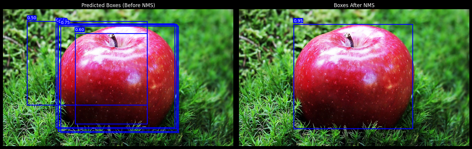
    plt.show()

Now, we visualize the bounding boxes before applying Non-Maximum Suppression:

draw_boxes_on_image(image, boxes, title='Predicted Boxes (Before NMS)')

Predicted Bounding Boxes Before NMS

5. Define IoU (Intersection over Union)

The Intersection over Union (IoU) metric is fundamental in NMS. It measures the overlap between two bounding boxes. If the overlap exceeds a certain threshold, one of the boxes will be suppressed.

def iou(box1, box2):
    x1 = max(box1[0], box2[0])
    y1 = max(box1[1], box2[1])
    x2 = min(box1[2], box2[2])
    y2 = min(box1[3], box2[3])

    inter_area = max(0, x2 - x1) * max(0, y2 - y1)
    box1_area = (box1[2] - box1[0]) * (box1[3] - box1[1])
    box2_area = (box2[2] - box2[0]) * (box2[3] - box2[1])

    union_area = box1_area + box2_area - inter_area
    return inter_area / union_area if union_area > 0 else 0

6. Implementing the NMS Algorithm

Now, we will implement the Non-Maximum Suppression algorithm. This function takes the list of boxes and applies the suppression based on the IoU threshold.

def non_max_suppression(boxes, iou_threshold=0.3):
    if len(boxes) == 0:
        return []

    boxes = boxes[boxes[:, 4].argsort()[::-1]]  # Sort boxes by confidence
    selected_boxes = []

    while len(boxes) > 0:
        chosen_box = boxes[0]
        selected_boxes.append(chosen_box)

        remaining_boxes = []
        for box in boxes[1:]:
            if iou(chosen_box, box) < iou_threshold:
                remaining_boxes.append(box)
        boxes = np.array(remaining_boxes)

    return np.array(selected_boxes)

This algorithm works by sorting the boxes based on their confidence score. The highest-scoring box is selected, and any boxes that have a high overlap (IoU) with it are removed. This process repeats until no boxes remain.

7. Apply NMS and Visualize the Final Result

Finally, we apply the NMS function and visualize the bounding boxes that remain after suppression.

nms_boxes = non_max_suppression(boxes, iou_threshold=0.3)
draw_boxes_on_image(image, nms_boxes, title='Boxes After NMS')

The resulting image will show only the most relevant bounding boxes, filtering out any redundant boxes that have high overlap with others. This is exactly how modern object detectors ensure that the predictions are clean and non-redundant.

Predicted Bounding Boxes After NMS

Understanding the Outcome

After applying NMS, we observe that:

• Only the bounding box with the highest confidence score remains for each cluster of overlapping boxes.

• The result is a cleaner and more reliable set of detections.

This filtering process is essential in real-world scenarios where object detectors may return hundreds of overlapping predictions.

Learn more about Object Detection with YOLO.

Conclusion

Non-Maximum Suppression is a fundamental concept in object detection. Although the idea is simple, its role is crucial for reducing noise in predictions and improving model accuracy.

By implementing it manually and visualizing the outcome, we gain a deeper appreciation of how object detectors work under the hood.

Understanding NMS equips you with the tools to customize detection outputs, debug model predictions, and experiment with alternative post-processing techniques.

All the code for this guide can be accessed on this GitHub Repository.