A 224×224 RGB image contains 150,528 numbers. Every computer vision system begins by turning pixels into arrays, and from that simple fact follow the practical decisions that shape a career: what to learn first, which dataset to practice on, and how to get a model to run outside a research lab.
By the end of this article you will have a concrete sequence of skills, tools, and projects that take you from writing your first image loader to shipping a small model that classifies or localizes objects. This is not an academic syllabus; it is a sequence of problems to solve and the minimum concepts needed to solve them well.
You do not need a PhD to build useful vision systems, but you do need a few tidy foundations. First: programming. Python is the industry standard because its ecosystem—NumPy, OpenCV, PyTorch, TensorFlow—lets you move from prototype to production quickly. Learn how to read and write images with OpenCV, manipulate arrays with NumPy, and build simple plots with Matplotlib. Spend ten focused hours building small utilities: an image resizer, a function that converts images to grayscale, and a script that reads a directory of labeled images into batches.
Second: linear algebra and probability, at a practical level. You should be comfortable with vectors and matrices, dot products, and the basics of eigenvalues because these concepts appear in everything from PCA to convolution. Probabilistic intuition—what a likelihood is, how loss functions relate to probability—makes classification and regression problems easier to reason about. You do not need proofs; you need to be able to translate a real task into a loss function you can minimize.
Third: image basics. Understand color spaces (RGB, HSV), common transformations (rotation, cropping, normalization), and why images are often resized to square tensors like 224×224 or 256×256. Learn how common augmentations change a dataset: random flips, color jitter, and rotation reduce overfitting by introducing variability. Try these augmentations on a small dataset to see how model performance changes.
A useful early rule: start with a pretrained convolutional neural network rather than building one from scratch. Convolutional networks detect local patterns—edges, textures, motifs—by applying small filters across an image. In practice, you will use models such as ResNet, MobileNet, or EfficientNet as backbones and then fine-tune them on your task. These models are available in libraries; importing a pretrained ResNet and training a classifier on top of it often produces good results in hours, not weeks.
Transfer learning is the pragmatic bridge between limited data and strong performance. If you have fewer than 10,000 labeled examples, freezing the early layers of a pretrained model and training only the last few layers is a fast, reliable approach. When you have 50,000–100,000 images, unfreezing and fine-tuning the whole network with a lower learning rate usually improves accuracy. Track validation loss and accuracy, and use early stopping to avoid overfitting.
For tasks beyond classification—object detection, semantic segmentation, instance segmentation—the architectures shift but the workflow is similar. Use a known detector like Faster R-CNN or a one-stage model like YOLO or EfficientDet for detection tasks. For segmentation, U-Net and DeepLab remain practical choices. Each of these models has trade-offs: two-stage detectors are more accurate but slower; one-stage detectors prioritize speed. Choose based on your application’s latency budget and hardware.
Good data beats clever models. Spend more time curating and labeling than obsessing over hyperparameters. Start with a small, well-labeled validation set of a few hundred examples that reflect the real deployment environment. Use that set to measure progress. When you change preprocessing, augmentation, or model depth, run controlled experiments and log results. If accuracy improves on training data but not on the validation set, you are overfitting; if both drop, you may have introduced a bug or misapplied augmentation.
ImageNet's training set contains roughly 1.2 million labeled images, which is why pretrained models trained on that corpus transfer so well to other tasks.
Label quality matters. A dataset with 5% mislabeled examples will cap your achievable accuracy, sometimes dramatically. For many projects, smart sampling for labeling—active learning, or labeling hard negatives first—reduces labeling effort. Tools such as LabelImg for bounding boxes and CVAT for video annotation remove friction from the process. If you need public datasets, explore the ImageNet dataset page, COCO for detection and segmentation, and Pascal VOC for compact benchmarks.
Compute decisions are practical constraints. Training a moderate ResNet on 50,000 images might take hours on a single GPU; training a large detector on a full dataset can take days on multiple GPUs. Cloud instances with GPUs cost between $0.50 and $4.00 per hour depending on the model. Budget accordingly and use mixed precision training and smaller batch sizes to accelerate experiments when possible.
Build projects that produce observable outputs. A classifier that sorts plant diseases from leaf photos is a compact, teachable project; a detector that finds defects on a manufacturing line demonstrates real-world constraints like occlusion and motion blur. Deploying a model reveals problems you won’t encounter in a notebook: input pipelines that drop frames, models that slow down when memory is fragmented, and distribution shift when the lighting in production differs from your training images.
Start with local deployment using a lightweight stack. Export a trained PyTorch model to TorchScript or ONNX and run inference with a CPU or an edge GPU such as a Jetson Nano. Measure end-to-end latency, including image capture and preprocessing. If your target is mobile, convert models to TensorFlow Lite or Apple’s Core ML formats and test on the device. For web deployment, WebAssembly and TensorFlow.js let you run models in the browser without server costs.
Monitoring matters. Once a model is live, track simple metrics: input distribution statistics, model confidence distributions, and task-specific KPIs such as precision at a fixed recall. Set up alerts for data drift—if the mean brightness of incoming images suddenly shifts, that is a signal to retrain. Periodically collect labeled examples from failure cases and fold them back into the training set; this feedback loop is the fastest way to improve real-world performance.
Practical projects teach more than tutorials. Work through one end-to-end project that includes labeling, training, and deployment. For a compact learning path: classify a dataset like CIFAR-10 to learn the tooling; fine-tune a pretrained ResNet on a custom dataset of a few thousand images; build and deploy a detector using a subset of COCO classes; instrument the deployed model and iterate based on real failures.
Keep an eye on libraries and resources that speed development. The PyTorch tutorials provide runnable examples for fine-tuning and detection. OpenCV’s documentation remains indispensable for preprocessing, feature extraction, and simple classical vision methods that often complement deep learning in low-compute settings.
Confidence grows through measurable iterations. Start small, measure carefully, and expand scope only after you can explain why a change improved performance. Each experiment should answer a single question: did this augmentation help, did this backbone reduce latency, did this labeling strategy reduce error? Over months, those answers compound into intuition that is more valuable than any single algorithmic trick.
Expect to repeat cycles of labeling, training, and deployment. Real-world vision projects are rarely solved in one pass; they are improved through successive refinements guided by concrete failure cases. As you accumulate projects—classifier, detector, and segmentation model—you will build a toolbox of patterns and an internal checklist for new problems: baseline with transfer learning, measure on a stable validation set, iterate with targeted labeling, and instrument production.
Learning computer vision is a series of small, concrete wins: your first correctly labeled dataset, your first model that runs at the required frame rate, your first reduction in false positives. Those wins stack into capability. Start with code that runs, add data that reflects reality, and prioritize experiments that give clear, measurable answers. That approach will get you from curiosity to production-ready models more reliably than chasing the newest architecture.